Available sampling methods
Risk Analysis offers you a choice of two sampling methods, which can be used to generate a different possible duration for each task for each iteration: Monte Carlo and Latin Hypercube.
What is sampling?
Sampling is the process by which values are taken randomly from a probability distribution - a range of possible values. Sampling takes place repetitively during risk analysis, as a different duration is selected for each task for every iteration, with each duration falling within the minimum and maximum duration range that has been specified for each task.
Risk Analysis supports four distributions. The examples in this topic are based on the use of a normal distribution, as illustrated below:
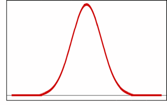
A probability distribution can be expressed as a cumulative curve, with the X axis representing the range of possible values - in the case of Risk Analysis, the range of possible durations that has been specified for a task - and the Y axis representing the cumulative probability of the corresponding values on the X axis. This is illustrated in the case of a normal distribution below:
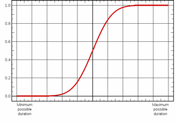
The shape of the cumulative curve differs depending on the distribution you choose to use.
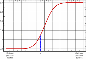
During a risk analysis iteration, for each task, a random number between 0 and 1 is generated. This random number is plotted on the Y axis of the cumulative probability distribution graph and used to select the corresponding value from the X axis. This is illustrated in the example below, where a random number of 0.3 is generated, resulting in duration x being sampled from the range of possible durations:
Plotted onto the normal distribution, the sampled value would appear as follows:
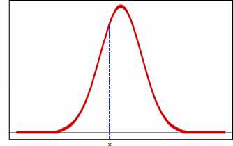
A different duration is sampled during each iteration that is performed.
The Monte Carlo sampling method
Using the Monte Carlo sampling method, a completely random number between 0 and 1 is generated for each iteration, plotted on the Y axis of the cumulative probability distribution graph and used to select the corresponding value from the X axis.
Because of the shape of the normal distribution's cumulative curve, the more likely outcomes - those possible durations in the range at which the cumulative curve is at its steepest - are more likely to be sampled using the Monte Carlo method. This is also the case if you use a skewed normal or skewed triangular distribution. If you perform a large number of iterations when carrying out risk analysis, this is not a problem, as the large number of iterations means that it is likely that the sampled durations cover the whole possible range. However, if you perform a small number of iterations, it is possible that the durations selected by the Monte Carlo method can 'cluster' around the area of the distribution that has a higher probability of occurrence. This can result in risk analysis under-representing the outcomes at the outer edges of the probability distribution.
A simplified example of this is illustrated in the following diagram, which shows the values selected during a risk analysis in which only five iterations are performed. In this example, the random numbers generated by the Monte Carlo method have all clustered around the area of the distribution that has a higher probability of occurrence, and the values in the outer ranges of the distribution are not represented at all:
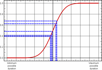
Plotted onto the normal distribution, these sampled values would appear as follows:
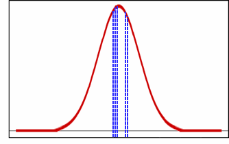
If you intend to perform a relatively small number of iterations when carrying out risk analysis, it is advisable to use the Latin Hypercube sampling method rather than Monte Carlo, as this method ensures that the sampled values are spread evenly across the whole distribution and avoids the potential problem of clustering.
The Latin Hypercube sampling method
Although the Monte Carlo sampling method has been proven to provide reliable results, as explained above, it can be less reliable when a small number of iterations are performed during risk analysis.
The Latin Hypercube sampling method gets around this problem. Using Latin Hypercube, the probability distribution is split into n segments of equal probability, where n is the number of iterations that are to be performed during risk analysis. As the risk analysis progresses, each of the n segments is sampled once (ie a random number is selected from within each segment), and only once.
For example, a risk analysis with 500 iterations would split the probability distribution into 500 segments, each representing 0.2% of the total distribution. For the first iteration, a random number between 0 and 0.2 would be generated, plotted on the Y axis of the cumulative probability distribution graph and used to select the corresponding value from the X axis; for the second iteration, a random number between 0.2 and 0.4 would be generated; and so on.
When a small number of iterations are performed, this has the advantage of generating a set of possible durations that more precisely reflects the shape of a sampled distribution than pure random (Monte Carlo) samples.
A simplified example of this is illustrated in the following diagram, which - as in the previous example - shows the values selected during a risk analysis in which only five iterations are performed. In this example, the Y axis of the cumulative probability distribution graph is split into five segments of equal probability. The splits occur on the Y axis at the 0.2, 0.4, 0.6 and 0.8 points and the segments are shaded using different colours. A random number is selected within each of these segments and used to select the corresponding value from the X axis:
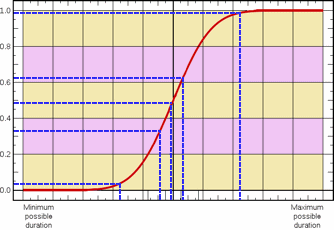
Plotted onto the normal distribution, these sampled values would appear as follows:
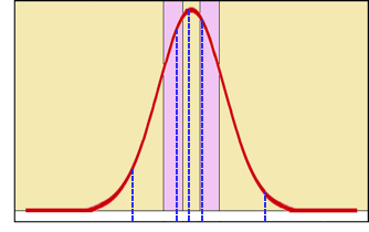
Given that Latin Hypercube sampling generates a set of values that more precisely reflects the shape of a distribution, it can be viewed as a more efficient sampling method than Monte Carlo in situations where fewer iterations are performed.
Sampling and the criticality index
As the durations sampled for each task differ from one iteration to another, tasks can appear on the critical path in some iterations but not in others. This is illustrated in the diagrams below.
The first diagram represents a project schedule containing three tasks: A, B and C. Three possible durations are shown for each task. The first figure is the minimum value in the range of possible durations, the second is the actual estimated duration of the task in the project and the third is the maximum value in the range of possible durations. All three tasks are currently on the critical path:

The overall time taken to complete all three tasks could be anywhere from 12 (2+7+3) to 27 (8+11+8).
In the following diagram, task D has been added to the project schedule:
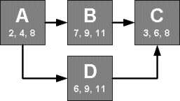
If risk analysis is performed again on the project, the durations selected for task B will sometimes be greater than those selected for task D, and vice-versa. Therefore the critical path will sometimes be A-B-C and sometimes A-D-C. The relative frequency of the alternative critical paths can tell you a lot about the nature of a project.
Risk Analysis records the percentage of time each task spends on the critical path during the simulation. This is known as a task's criticality index. The criticality index is a measure of the importance of a task within a project: the higher the criticality index, the more important the task and the more likely the task is to affect the finish date of the project.
Estimating the duration uncertainty and probability of tasks